

Table des matières
The objective of this TD is: (1) to learn how to use numpy to carry out efficient calculations and (2) to have a better understanding of matplotlib.
When is numpy effective?
List of lists
The following code:
- creates a randomly generated list of lists
A, containing a large number of0and1; - makes a second list of lists, having the same size as
A, which we subtly callB; - copies the values from
AtoB.
We can measure the execution time of the computation of the values of the matrix B. We should obtain a time of the order of a few hundredths of seconds. Test it.
from random import randint
from timeit import timeit

A = [[randint(0,1) for _ in range(300)] for _ in range(600)]
B = [[0 for _ in range(300)] for _ in range(600)]

def copy(A, B):
    for i in range(0, len(A)):
        for j in range(0, len(A[0])):
            B[i][j] = A[i][j]

timeit("copy(A, B)", number=10, globals=globals())
Numpy array
The following code is used to do an equivalent operation using numpy. Compare its execution time with the one obtained before. Does this surprise you?
import numpy as np

A = np.random.randint(0, 2, (300, 600))
B = np.zeros(A.shape)

def copy(A, B):
    for i in range(0, len(A)):
        for j in range(0, len(A[0])):
            B[i,j] = A[i,j]

timeit("copy(A, B)", number=10, globals=globals())
The good way
It seems that the use of numpy leads to poorer performances than the use of lists.
The problem here is that we are not using numpy properly. Indeed, this library is optimized for "vectorization" or "array programming". It is a technique of applying operations to one set of data at a time.
We need to change our approach to take fully advantage of numpy.
For example, the correct way to perform a copy operation is the following.
You should agree that it is significantly more efficient.
A = np.random.randint(0, 2, (300, 600))
B = np.zeros(A.shape)

def copy(A, B):
    A[:,:] = B[:,:]

timeit("copy(A, B)", number=10, globals=globals())
How to use Numpy
Slice of lists
You already know how to slice lists. Here is an example, we note that :
- when slicing is used to the left of an equal sign, it is used to set values in a list;
- when slicing is used to the right of an equal sign, it is used to duplicate a part of a list.
l = [0, 1, 2, 3, 4, 5]
print("Id of l  : ", id(l))
l[:3] = [2, 1, 0]
print("l :  ", l)

l2 = l[:4]
print("Id of l2 : ", id(l2))  #Two python objects with the same id are physically the same
l2[:] = [0, 0, 0, 0]          #Warning do not confuse with "l2 = [0, 0, 0]" which is used to change the reference l2
print("Id of l2 : ", id(l2))

print("l :  ", l)
print("l2 : ", l2)
Views
Using the same notation on a numpy array does not create a slice. Instead, it creates a view, which is another way of viewing the data, but it is not a copy of the data.
Test the following code.
L = np.array([0, 1, 2, 3, 4, 5])
print("Id of L  : ", id(L))
L[:3] = [2, 1, 0]
print("L :  ", L)

L2 = L[:4]
print("Id of L2 : ", id(L2))  #Two python objects with the same id are physically the same
L2[:] = [0, 0, 0, 0]          #Warning do not confuse with "L2 = [0, 0, 0]" which is used  to change reference L2
print("Id of L2 : ", id(L2))

print("L :  ", L)
print("L2 : ", L2)
Arrays and views can often be used indifferently. When handling a view, the base attribute points to the corresponding array.
print("Base of L :  ", L.base)
print("Base of L2 : ", L2.base)

print("Id of L : ", id(L))
print("Id of the base of L2 : ", id(L2.base))
A view is a link to data and an organization of data. With reshape we can create new views towards data which can be organized differently.
L3 = np.reshape(L2, (2, 2))
L3[1, 0] = 9
print("L3 :\n", L3)
print("L :\n", L)
Indexing
It is possible to reference indices as in slices (start, end, step); however, when handling numpy arrays with several dimensions, it is not necessary to chain the brackets to access lists of lists (of lists...), you can just use commas.
Finally, we can assign the values contained in a view using another view of the same size and same dimension, or a scalar.
For more informations: indexing
A = np.ones((3, 4))
print("Array A :\n", A)

A[::2, :] = 2
print("Array A: modified with a scalar\n", A)

B = np.zeros((3, 4))
A[:,:] = B[:,:]
print("Array A: modified with a view\n", A)
Photo editing
Warning: We want to answer the following questions using vectorization. You must never use loops explicitly. We provide "useful functions" for each question; they are necessary, but not always sufficient.
We can read PNG images with matplotlib and return a three-dimensional array that contains the intensity of each color of each pixel. The intensity is a value between 0 and 255.
- dimension 1 is the abscissa of a pixel;
- dimension 2 is the ordinate of a pixel;
- dimension 3 is the color index, in RGB format.
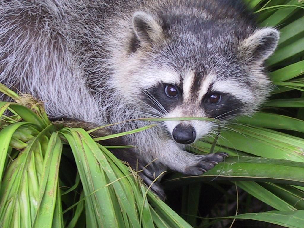
We chose this raccoon image because it allows us to correctly visualize the processing that we're about to describe.
Download the image and save it to your working directory.
After testing your functions on this image, you may very well use other PNG images.
Depending on your computer (and the libraries installed), imread() may have a slightly different behavior. In particular :
- it can return an array of integer values (between 0 and 255), or an array of floating-point numbers (between 0. and 1.);
- the last dimension of the array can be of dimension 3 or 4; (in the latter case, each pixel is encoded in the RGBA format: red, green, blue and transparency).
The remainder of the questions assume that you have an array of integer numbers and the last dimension is 3. If that's not the case for you, please uncomment the two corresponding lines (look at the comments) in the following code:
import matplotlib.pyplot as plt
import numpy as np


img = plt.imread("raccoon.png")
#Convert to int
#img = img * 255
#img = img.astype(int)

#Remove the transparency component
#img = img[:,:,0:3]
plt.imshow(img, norm=None)
plt.show()
Grayscale
Conversion
Write a function grayscale(img) which takes as a parameter a color image in the form of an array and returns a new array of only 2 dimensions, containing the gray level of each pixel.
Our eyes do not perceive the luminous intensity of each color in the same way, it is necessary to apply the following coefficients for the conversion: red 30%, green 59% and blue 11%.
Here are some useful functions / operations:
A * x, the operation multiplies each value ofAby the scalarx;A.astype(int), creates a copy of the arrayAcontaining only rounded values;plt.imshow(img, cmap="gray")displays a grayscale image.
Histogram
Write a function histogram(img) which takes a grayscale image as a parameter and returns a histogram of the values of the intensities present in the image. The return value is therefore a numpy array of 256 values between 0 and 1, representing the proportion of pixels having a certain value.
Here are some useful functions:
A / x: it divides, in place, each value ofAby the scalarx;np.zeros(n): it creates a one-dimension array of sizen;np.add.at(A, indices, x)for each valueiin the arrayindices, increments byxthei-th value ofA; It is equivalent to something likefor i in indices: A[i] += xbut faster.np.sum(A)sums the list of elements inA.
Plot histogram
Write a function plot_intensity(img) that displays an image and the histogram of the intensities side by side.
Here are some useful functions:
np.linspace(0, 255, 256)creates a new array with 256 values evenly distributed between 0 and 255 (inclusive);plt.fill_between(x, y)plots a filled solid curve;plt.subplots(figsize = (15, 5))creates a multiple graph of a given size;plt.subplot(nbr, nbc, num)indicates the location of the next curve to plot. Example of subplot : click here.
Contrast
A photo is considered to be correctly exposed if the intensities are well distributed over the whole spectrum, in particular, the black must be deep and the white very bright. Many image editing tools allow us to automatically choose the contrast and the brightness to obtain a balanced image.
A naive approach to achieve this operation consists in transforming the 2% of the lowest intensities in absolute black (value of 0) and the 2% of the strongest light intensities in a saturated white (value of 255). The intermediate values are distributed linearly.
The first step, therefore, consists in finding the values {$p_2$} and {$p_{98}$} from the 2nd and 98th centiles. In other words, {$p_2$} is the intensity such that 2% of the total intensities are lower. The values {$p_2$} and {$p_{98}$} are between 0 and 255.
Once these values are known, it is possible to solve the following equation system, where {$C$} and {$I$} refer to the contrast and intensity corrections: {$$C*p_2 + I = 0$$} {$$C * p_{98} + I = 255$$}
Once this system is solved, it is possible to correct each value {$i$} of intensity of the grayscale image by the new intensity : {$C*i + I$}.
Centiles
Write a function centile(img) which, given a grayscale image, computes and returns the 2nd and 98th centiles.
np.percentile(A, x)computes the x-th percentile of A.
You can use the above function or, exceptionally, you can use a for loop on the histogram. The result for the racoon should be (11, 213) (or similar values).
Solving the system
Numpy provides a module to solve linear systems of equations. Equations must be expressed as matrices.
{$$ \left( \begin{matrix} p_2 & 1 \\ p_{98} & 1 \end{matrix} \right) * \left( \begin{matrix} C \\ I \end{matrix} \right) = \left( \begin{matrix} 0 \\ 255 \end{matrix} \right) $$}
Write a function find_corrections(img) that returns the contrast and intensity corrections to be made. Here are the helpful instructions:
from numpy import linalgX = linalg.solve(A, B)with AX = B
Auto constrast
Write a function auto_contrast(img) that takes a grayscale image as a parameter and returns a new image with the application of the automatic contrast algorithm.
Here are some useful functions:
np.zeros_like(A)creates a new array of the same shape and size asAand containing zeros;np.clip(A, min, max)creates a new array where values inAless thanminare replaced byminand those greater thanmaxare replaced bymax.
Well done
You have completed this TD. Now you know how numpy views work and how to use numpy to avoid explicit loops. If you still have time, you might want to answer the following questions.
Optional questions - Color image
Color histogram
Write a function plot_color_intensities(img) which displays an image and, next to it, the 3 intensity histograms (R, G and B) superposed. We can use the function histogram(img) that we previously created to retrieve the intensity histogram of a grayscale image and apply it to a view of each color.
Useful function:
plt.fill_between(x, y, color="#FF000055")to display a filled red solid curve (hexadecimal notation color codes).
Color model conversion
Our image is currently encoded with the RGB color model. In this model the intensity is "distributed" over each of the three colors. We could imagine an auto-contrast algorithm on color images by working on each intensity independently. By doing so, we take the risk of changing the hue of an image.
For auto-contrast it is better to change the color model, for example the YCbCr model. In this model, each pixel is represented by three components. The first Y is intensity (0 for black, 255 for white). The second and third components represent the variation in hue.
We can switch from the RGB model to the YCbCr model:
{$$ \left( \begin{matrix} Y \\ C_b \\ C_r \end{matrix} \right) = \left( \begin{matrix} 0 \\ 128 \\ 128 \end{matrix} \right) + \left( \begin{matrix} 0.299 & 0.587 & 0.114 \\ −0.168736 & −0.331264 & 0.5 \\ 0.5 & −0.418688 & −0.081312 \end{matrix} \right) * \left( \begin{matrix} R \\ G \\ B \end{matrix} \right) $$}
and conversely
{$$ \left( \begin{matrix} R \\ G \\ B \end{matrix} \right) = \left( \begin{matrix} 1 & 0 & 1.402 \\ 1 & −0.344136 & −0.714136 \\ 1 & 1.772 & 0 \end{matrix} \right) * \left( \begin{matrix} Y \\ C_b-128 \\ C_r-128 \end{matrix} \right) $$}
Write two functions to_YCbCr(img) and to_RGB(img) to switch from one model to another. Also write a function test_conversion(img) which checks that everything is in order (if this is the case, the difference between each pixel of an image img and to_RGB(to_YCbCr(img)) should be small (less than 1 if you forget that the values are integer, a few units otherwise).
Tips: The matrix to convert a pixel is of dimension (3, 3). However, an image is of dimension (rows, cols, 3). The numpy documentation says about the np.dot(a, b) product function: "a sum product over the last axis of a and the second-to-last of b". The simplest solution is therefore to reverse the order of the operands of the product and therefore to transpose the conversion matrix.
Here are some useful functions:
np.dot(A, B), product;A.Tis the transpose ofA;A.astype(int)builds an array with rounded values ofA;np.clip(A, 0, 255)builds an array with the values in the interval [0,255];np.absolute(A)builds an array with the absolute values of A.
Color auto constrast
Write a function auto_contrast_YCbCr(img) which converts img in YCbCr mode, applies auto contrast to the Y component, then returns the converted image in RGB mode.