Table of contents
First Laboratory Session
The two laboratory sessions sessions of the Algorithmics and Complexity module are a small programming project. The problem to be solved is a land planning for ensuring access to a health care service. The goal is to place a certain number of hospitals in order to cover a territory at best.
Objectives of the TP
The work carried out during the two 3-hour practical sessions, completed possibly through personal work between the two sessions, has the following objectives:
- To allow students to program classical algorithms seen in class:
- graph search algorithm
- shortest path algorithm
- greedy algorithm
- random algorithm
- brute force algorithm (course 8)
- To implement an environment and programming tools for the resolution of the problem:
- reading entries
- generation of random input sets
- definition of metrics and realization of benchmarks.
- display of inputs and outputs
Practical information
The development will be done under Python using an IDE with a debugger, such as Visual Studio Code that you used in the course of programming in the first sequence (SIP in SG1) and you learned to debug with it.
For each exercise, after having written the Python code of the requested function, you must also define a function to test and call this code named Q_N() (N being the number of the question). The call of Q_N() can thus be commented in the code when doing the next exercises.
You must have completed questions 1 to 7 before the second session.
Definition of the problem
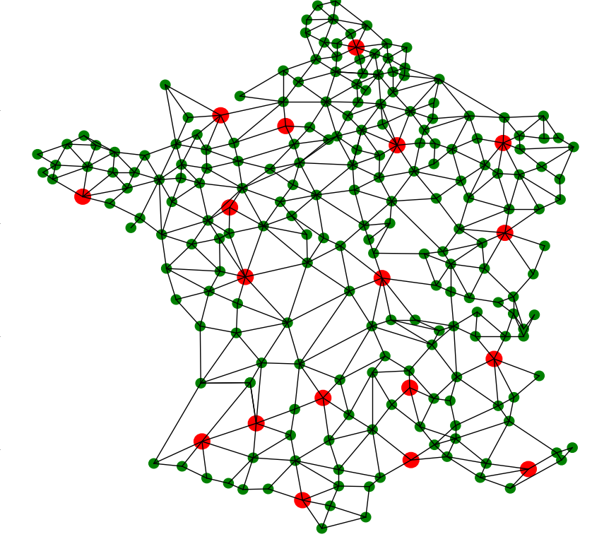
The objective of the project is to write a program that allows one to choose the city (or the cities) in which we set up hospitals to cover an entire area at best.
Input data is therefore :
- a set of cities linked by roads;
- a subset of candidate cities to host a hospital (not all cities can host a hospital).
The program has to produce a subset of candidate cities such as each city in the territory has either a hospital or is "covered" by a hospital of another city. This notion of coverage will be detailed in the second lab session. The idea is to take into account the distance between a city and the nearest hospital.
The program will also have a graphical user interface that allows us to display the result.
Data representation
We will define a data structure to represent our maps/cities in memory. This data structure must be adapted to be used in our algorithms and to be displayed in the graphical interface.
We will also need to import the map of the territory provided to the program as a file.
Map of the territory in memory
To represent the map of the territory in memory, we will use a Python dictionary.
Each city will be represented by a dictionary's entry whose key is the name of the city (a string) and the value is also a dictionary composed of two entries indexed by the following keys:
- coords : the Cartesian coordinates of the city on the map;
- next : the list of neighbors with their distances, which will again be a dictionary whose keys are the names of neighboring cities and the values are the distances (i.e. lengths of roads) to these cities.
Consequently, a map may be presented as:
map = {
       'La Baule-Escoublac':{'coords':(356, 638),
                            'next':{'Saint-Nazaire':15, 'Guérande':6, 'Saint-André-des-Eaux':8}},
       'Saint-Nazaire':{'coords':...},
       ...
}
Observe three nested dictionaries. The use of dictionaries (unlike lists) allows an optimal access time in {$\mathcal{O}(1)$}
Map of the territory as a file
The map of the territory will be provided to you in a file composed of two parts separated by a line containing two dashes: --. The first part contains the list of cities and their Cartesian coordinates. The second part of the file contains the list of direct connections between the cities and the distances of the roads between them, for instance:
La Baule-Escoublac:356:638
Saint-Nazaire:484:563
Guerande:180:340
Saint-André-des-Eaux:345:402
--
La Baule-Escoublac:Saint-Nazaire:15
La Baule-Escoublac:Guérande:6
La Baule-Escoublac:Saint-André-des-Eaux:8
To load a map from a file, you can use the following code :
def read_map(filename):
    f = open(file=filename, mode='r', encoding='utf-8')

    map = {}
    while True:  # reading list of cities from file
        ligne = f.readline().rstrip()
        if (ligne == '--'):
            break
        info = ligne.split(':')
        map[info[0]] = {'coords': (int(info[1]), int(info[2])), 'next':{}}

    while True:  # reading list of distances from file
        ligne = f.readline().rstrip()
        if (ligne == ''):
            break
        info = ligne.split(':')
        map[info[0]]['next'][info[1]] = int(info[2])
        map[info[1]]['next'][info[0]] = int(info[2])

    return map
Toy example
Create a tp.py file in your development environment and copy the toy example provided below (the toy_map dictionary) into it:
toy_map = {'A': {'coords': (100, 100), 'next': {'B': 140, 'E': 200, 'F': 200}},
           'B': {'coords': (200, 140), 'next': {'A': 140, 'C': 260, 'F': 140}},
           'C': {'coords': (360,  40), 'next': {'B': 260, 'D': 360}},
           'D': {'coords': (320, 360), 'next': {'C': 360, 'F': 280}},
           'E': {'coords': ( 80, 280), 'next': {'A': 200, 'F': 120}},
           'F': {'coords': (160, 240), 'next': {'A': 200, 'B': 140, 'D': 280, 'E': 120}} }

assert read_map('territoire_jouet.map') == toy_map
This territory corresponds to the data contained in the file territoire_jouet.map available here. Download this file and save it in your working directory. Check that the map loaded from territoire_jouet.map corresponds to toy_map.
Graphical visualization
We keep the tkinter library that you used during the programming course in SG1. To display a map in a graphical window, we provide you with the function draw_map(map, hospitals = []) which takes as parameters :
 - map : the dictionary representing the map in the memory format detailed in the previous section ;
 - hospitals: a Python list of the names of the cities hosting a hospital. These cities will be colored in red. This parameter is optional ;
 - l and h : the width and height of the display window, which should be sufficient to display all cities whose coordinates correspond to pixels.
Test the following code:
import tkinter as tk
def draw_map(map, hospitals = [], l = 800, h = 800):
w = tk.Tk()
c = tk.Canvas(w, width=l, height=h)
for city in map:
for vname in map[city]['next']:
if city < vname:
x1 , y1 = map[city]['coords']
x2 , y2 = map[vname]['coords']
c.create_line(x1, y1, x2, y2, dash=True)
c.create_text((x1+x2)//2, (y1+y2)//2, text=map[city]['next'][vname])
for city in map:
x , y = map[city]['coords']
color = 'red' if city in hospitals else 'black'
c.create_rectangle(x-5, y-5, x+5, y+5, fill=color)
c.create_text(x+12, y+12, text=city)
c.pack()
w.mainloop()
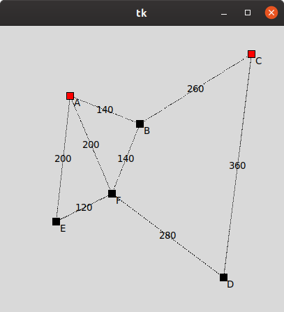
draw_map(toy_map, ['A', 'C']) # remember to comment this line after the test
The result obtained should be as follows:
Automatic generation of maps
In order to be able to feed the implemented algorithms with data and make benchmarks to compare their performance, we need maps of different sizes (i.e. number of cities) and different densities (i.e. number of roads).
The function random_grid_map(n, step) takes as parameters two integers n and step and returns a square grid of {$n \times n$} cities. The coordinates of the cities (the unit is the pixel) are spaced by the step step% and each edge of the grid is labelled with a distance (an integer value) randomly drawn in the open interval {$]step, 2 \times step [$}.
import random

def random_grid_map (n, step):
    map = {f'{i}_{j}': {'coords':(j*step,i*step), 'next':{}} for i in range(1, n+1) for j in range(1, n+1)}

    for i in range(1, n+1):
        for j in range(1, n):
            d = random.randint(step+1, 2*step)
            map[f'{i}_{j}']['next'][f'{i}_{j+1}'] = d
            map[f'{i}_{j+1}']['next'][f'{i}_{j}'] = d

    for i in range(1, n):
        for j in range(1, n+1):
            d = random.randint(step+1, 2*step)
            map[f'{i}_{j}']['next'][f'{i+1}_{j}'] = d
            map[f'{i+1}_{j}']['next'][f'{i}_{j}'] = d

    return map

draw_map(random_grid_map(5,100))
For example, an execution of random_grid_map (5, 100) should generate a map as displayed below, only distances can vary :
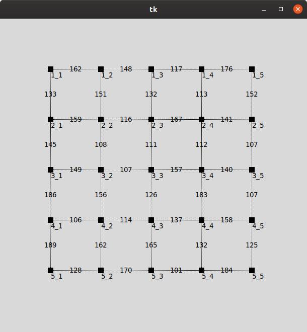
The random_grid_map function generates a connected but a non-dense graph as {$|E| < 2|V|$}. A dense graph would have {$|E| \approx |V|^2$}.
Write a function random_dense_map(n, d_max) that takes as parameters two integers n and d_max and generates a map which is a complete graph with {$n$} distinct cities and {$\frac{n \times (n-1)}{2}$} edges. The coordinates of the cities as well as the distances of the edges are integer values drawn randomly in the open interval {$]0, d_{max}[$}.
You can use the following check_map(map) function to verify that your generated map is well formed:
def check_map(map, complete=False):
    for city in map:
        for neighbor in map [city]['next']:
            if neighbor not in map:
                print('Error: The neighbor', neighbor, 'of the city', city, 'does not exist')
                return False
            if city not in map [neighbor]['next']:
                print('Error: The city', city, 'and the city', neighbor, 'are not reciprocally neighbors')
                return False
            if map [city]['next'] [neighbor] != map [neighbor]['next'] [city]:
                print('Error: The city', city, 'and the city', neighbor, 'are not at the same distance reciprocally')
                return False
        if complete:
            if len(map[city]['next']) < len(map) - 1:
                print('Error : The graph is not complete, there are missing neighbors to :', city)
                return False
    return True

def Q_1():
    complete_map = random_dense_map(10,500)
    assert len(complete_map) == 10 and check_map(complete_map, complete=True)
    draw_map(complete_map)
Computing the shortest paths
In the next part of the topic, we will need to compute the shortest distances between cities. We will use the algorithm of the shortest paths from a source s. This algorithm was invented by one of the fathers of computer science: Edsger Dijkstra.
We are only interested in calculating the distances between s and other cities: the path is not important for our problem.
Below is the Python version of the algorithm as presented in lecture 2, in which we have removed the parent dictionary. PCCs stands for Plus Courts Chemins in french.
def PCCs(graph,s):
    frontier = [s]
    dist = {s: 0}

    while len(frontier)>0:

        ### extraction of the node of the boundary having the minimum distance ###
        x = extract_min_dist(frontier,dist)

        ### for each updated neighbor of the border and its distance ###
        for y in neighbors(graph, x):
            if y not in dist:
                frontier.append(y)

            new_dist = dist[x] + distance(graph,x,y)
            if y not in dist or dist[y] > new_dist:
                dist[y] = new_dist

    return dist
In lecture 2 we discussed the impact of the data structure chosen to represent the frontier on the algorithm performance. We remind you that the complexity of such an algorithm is {$\mathcal{O}(|V|\times C_{extract\_min}\,+\,|E|\times C_{update})$}.
In the version above, this is the naive implementation where we use an unsorted Python list to represent the frontier. We want to compare it with an implementation where we use a binary heap ({$heap_{min}$}) to represent the frontier. Remember that each implementation has different {$C_{extract\_min}$} and {$C_{update}$} complexities. We also remind that the choice of data structure determines whether the worst case complexity of the algorithm depend or not on the density of the graph. The following table summarizes the set of worst-case complexities already analyzed in lecture 2.
| naive implementation | binary heap | |
| {$C_{extract\_min} = \mathcal{O}(|V|)$} | {$C_{extract\_min} =\mathcal{O}(log(|V|))$} | |
| {$C_{update} = \mathcal{O}(1)$} | {$C_{update} = \mathcal{O}(log(|V|))$} | |
| {$C_{PCCs} = \mathcal{O}(|V|^2 + |E|)$} | {$C_{PCCs} = \mathcal{O}((|V|+|E|)\log|V|)$} | |
| non-dense graph {$|E|\approx|V|$} | {$\approx \mathcal{O}(|V|^2)$} | {$\approx \mathcal{O}(|V|\log|V|)$} |
| very dense graph {$|E|\approx|V|^2$} | {$\approx \mathcal{O}(|V|^2)$} | {$\approx \mathcal{O}(|V|^2\log|V|)$} |
We propose to verify experimentally these worst case complexities inputting randomly generated maps with different densities.
Naive implementation.
Write a PCCs_naive version of the PCCs code above, replacing the extract_min_dist(frontier, dist) function with a code that returns the element with the minimum distance value. The frontier here is a simple Python list. Do not forget to implement neighbors(graph,x) and distance(graph,x,y) too.
Test the computed shortest paths of the toy territory when taking 'A' as the starting city :
def Q_2():
    assert PCCs_naive(toy_map, 'A') == {'A': 0, 'B': 140, 'E': 200, 'F': 200, 'C': 400, 'D': 480}
Binary heap
The standard Python library includes the module heapq (documentation here) which provides us with the heap data structure. This library is installed by default.
After reading the documentation, play with the following example :
from heapq import *

tas = [(1,'a'), (2,'b')]      ### the french word for heap is 'tas'
heapify(tas)               ### create a min heap from any list in O(n)
heappush(tas, (0,'c'))      ### inserting in O(log n)
print(heappop(tas))        ### extraction of (0, 'c') in O(log n)
print(heappop(tas)[0])     ### extraction >>> '1'.
print(len(tas))            ### measure in O(1) >>> 1
print(heappop(tas)[1])     ### extraction >>> 'b'
With heapq we have the insertion and extraction primitives but we have no primitive to change the priority of an element in the heap. Such an update is necessary in the implementation of the shortest path algorithm because the distance of a node that is part of the frontier can be improved if it is close to the current node and the latter offers a shorter path.
Updating a heap element is a primitive that is rarely necessary when using priority queues. This is the reason why it is often missing from libraries. This primitive is simple to implement, but it requires to maintain a dictionary associating a key to its position in the array representing the heap. Even if this can be done in constant time, it is a constant that slows down the implementation for many cases that do not require this primitive.
Other modules exist in Python such as HeapDict implementing heaps with this updating feature, but they require installation. We will therefore adapt to heapq which also has the advantage of being very efficient in terms of perfomence. Our strategy is as follows:
- Since update in a heap is not available, we will accept that a node is added several times to the frontier (min_heap), i.e. each time its distance is updated;
- A node is processed when it is extracted from the frontier for the first time;
- If the same node is extracted from the frontier again, it will be ignored and the next node will be extracted.
This change will have an impact on the size of the heap, which will go from a maximum size of {$|V|$} elements to potentially {$|E| \approx |V|^2$} elements if the graph is dense. The impact on performance remains, however, minimal since insertion and extraction will stay in in {$\mathcal{O}(log(|E|)) \approx \mathcal{O}(log(|V|))$}.
Write a function PCCs_heap(map, s) that takes as an argument a map map and a starting city s and returns the distance dictionary using heapq and applying the stated strategy.
Check that this function returns the right table for the toy territory:
def Q_3():
    assert PCCs_heap(toy_map, 'A') == {'A': 0, 'B': 140, 'E': 200, 'F': 200, 'C': 400, 'D': 480}
To check if a node has already been extracted, use a Python set or a Python dictionary to search in {$\mathcal{O}(1)$}. If you use a simple list the search will cost {$\mathcal{O}(|V|)$}!
Calculation of all the shortest paths
Write a function all_distances(map, PCCs = PCCs_heap) which takes as a parameter the map of the territory and a function computing the shortest paths (we use heaps by default), and which calculates the distances between any couple of cities. These distances are grouped in a dictionary whose keys are pairs of cities.
The value returned by the call of the function all_distances on the toy territory is the following symmetrical table:
assert all_distances(toy_map) == {('A', 'A'):   0, ('A', 'B'): 140, ('A', 'C'): 400, ('A', 'D'): 480, ('A', 'E'): 200, ('A', 'F'): 200,
                                  ('B', 'A'): 140, ('B', 'B'):   0, ('B', 'C'): 260, ('B', 'D'): 420, ('B', 'E'): 260, ('B', 'F'): 140,
                                  ('C', 'A'): 400, ('C', 'B'): 260, ('C', 'C'):   0, ('C', 'D'): 360, ('C', 'E'): 520, ('C', 'F'): 400,
                                  ('D', 'A'): 480, ('D', 'B'): 420, ('D', 'C'): 360, ('D', 'D'):   0, ('D', 'E'): 400, ('D', 'F'): 280,
                                  ('E', 'A'): 200, ('E', 'B'): 260, ('E', 'C'): 520, ('E', 'D'): 400, ('E', 'E'):   0, ('E', 'F'): 120,
                                  ('F', 'A'): 200, ('F', 'B'): 140, ('F', 'C'): 400, ('F', 'D'): 280, ('F', 'E'): 120, ('F', 'F'):   0}

map_grid = random_grid_map(10,100)
assert all_distances(map_grid, PCCs_heap) == all_distances(map_grid, PCCs_naive)

map_dense = random_dense_map(100,1000)
assert all_distances(map_dense, PCCs_heap) == all_distances(map_dense, PCCs_naive)
You will use the random map generators to test that the function all_distances returns the same table of distances with the function PCCs_heap as with the function PCCs_naive.
Benchmark
The Python module timeit allows one to measure the execution time of a Python function passed as a parameter and launched number times.
Using the following code, compare the execution time of the two versions {$naive$} and {$heap$} of the shortest paths computations.
import matplotlib.pyplot as plt
from timeit import timeit

def benchmark():
    Time_heap_grid = []
    Time_naive_grid = []
    Time_heap_dense = []
    Time_naive_dense = []

    n_list = []

    for N in range(10, 25):
        print(N) # to follow its running

        n = N*N
        n_list.append(n)

        # we compare on non-dense maps: grid of side N contains N*N cities
        map_grid = random_grid_map(n = N, step = 100)

        # an average is calculated over N launches by randomly selecting a starting city each time
        Time_naive_grid.append(timeit(lambda: PCCs_naive(map_grid, random.choice(list(map_grid))), number=N) / N)
        Time_heap_grid.append(timeit(lambda: PCCs_heap(map_grid, random.choice(list(map_grid))), number=N) / N)

        # we compare on dense maps
        map_dense = random_dense_map(n = N*N, d_max = 10000)

        Time_naive_dense.append(timeit(lambda: PCCs_naive(map_dense, random.choice(list(map_dense))), number=N) / N)
        Time_heap_dense.append(timeit(lambda: PCCs_heap(map_dense, random.choice(list(map_dense))), number=N) / N)

    plt.subplot(2, 1, 1)
    plt.xlabel('N')
    plt.ylabel('T')
    plt.plot(n_list, Time_naive_grid, 'r^', label='naive grid')
    plt.plot(n_list, Time_heap_grid, 'b^', label='heap grid')
    plt.legend()

    plt.subplot(2, 1, 2)
    plt.xlabel('N')
    plt.ylabel('T')
    plt.plot(n_list, Time_naive_dense, 'r*', label='naive dense')
    plt.plot(n_list, Time_heap_dense, 'b*', label='heap dense')
    plt.legend()

    plt.show()
Based on the table of complexities detailed above:
- the naive implementation must have a similar behavior between dense and non-dense maps.
- binary heap implementation should have lower performance on dense maps and better performance on non-dense ones.
What do you observe in this benchmark? Surprising!
Note: Discuss this with your TD supervisor. Write your answer as a comment in your source file.
help
The worst case complexity calculation takes {$|E|$} as the number of updates and {$|V|$} as the frontier size!
[to go further] motivated students will be able to instrument their codes to measure the quality of these assumptions by empirically calculating the average size of the frontier and the real number of updates.
List of candidate cities
Do not forget that our goal is to write a program that allows you to choose the city or the cities where hospitals should be located to cover the territory. From a description of the territory and a list of candidate cities, the program must select a subset of the candidate cities such that each city in the territory is either hosting a hospital, or covered by a hospital of another city.
To do this, we will now write a function which lists all the possible solutions, i.e. all the possible solutions are combinations of candidate cities. This function will be used in the second lab session in the implementation of the backtracking and approximation algorithms.
A combination is a sub-list of candidate cities. For example, if our candidates are ['A', 'B', 'C', 'D'], we have {$2^4 = 16$} combinations to cover the territory:
[]
['A']
['B']
['A', 'B']
['C']
['A', 'C']
['B', 'C']
['A', 'B', 'C']
['D']
['A', 'D']
['B', 'D']
['A', 'B', 'D']
['C', 'D']
['A', 'C', 'D']
['B', 'C', 'D']
['A', 'B', 'C', 'D' ]
A simple technique to get all the combinations is to enumerate all the numbers from {$0$} to {$2^n$} where n = len(candidates) using their binary representation. See like that a city is associated to a bit.
Write a function all_combis(candidates) that displays (print) all the combinations of elements of a list candidates passed in parameter.
In this algorithm, the combinations will be displayed on the fly: we do not keep in memory the list of all the combinations. combinations, as its size would be exponential!
help
Use Python binary AND(&). For example n & (2**i) allows to test if the {$i^{th}$} bit of n is at 1.
Generators
We want to iterate with a loop for on the combinations of candidate cities without going through a list of exponential size. We should transform the function all_combis(candidates) into a generator.
Without going into too much detail, this is possible with the use of the keyword yield which allows one to "resume" the execution of the function where it was left at each iteration of the loop for.
Replace the instruction print in all_combis(candidates) with a yield to obtain a generator that can be used in the following way :
for combi in all_combis(candidates):
    ...
Only {$k$} hospitals can be built with the available funding. For this reason we will generate the combinations of size {$k$} only.
Write a generator all_combis_k(candidates, k) that generates only the combinations of exact size k from the candidates list.
Test it with the following code :
for combi in all_combis_k(['A','B','C','D'], k=2):
    print(combi)

fake_candidates = [f'city{i}''' for i in range(50)]
for combi in all_combis_k(fake_candidates, k=1):
    print(combi)
Use Ctrl + C to stop it, what do you observe?
To go further...
The exercises in this last part of the first lab are optional: they use concepts that we will see in more details in lecture 8. If you have completed the previous exercises before the end of the first lab session, you can take advantage of these optional exercises.
To overcome the problem you have just observed, we will change the algorithm for enumerating all the combinations and we will use an implicit graph. An implicit graph is a graph of which we build the necessary parts as the search continues. As we will see later, this technique is often used when exploring state spaces (see lecture 8).
Neighborhood of a combination
We are going to represent the space of the combinations of the candidate cities by an oriented graph in which each node is a pair of lists:
- a list of the cities already chosen and which corresponds to the beginning of a possible combination
- a list of cities that are still candidates
To create the neighborhood of each node, we extend the list of selected cities with an additional candidate city from the second list. A node thus has as many neighbors as there are cities in its second list of candidate cities.
For example, the node (['A','C'], ['B','D','E']) represents the combination of size two which chooses 'A' and 'C' and has three neighboring nodes where each adds one city among the still candidate cities ['B','D','E'].
Write a generator neighbors(node_combi) that displays the neighbors of the node node_combi. For example:
for v in neighbors((['A', 'C'], ['B', 'D', 'E']):
    print(v)

>>> (['A', 'C', 'E'], ['B', 'D'])
     (['A', 'C', 'D'], ['B'])
     (['A', 'C', 'B'], [])
With such a neighborhood relation and starting from the empty combination ([], candidates), we can see that the unfolded implicit graph corresponds to a tree of {$2^n$} nodes where each node corresponds to a different combination.
Exploring the combination tree
We now want to write a generator combi_gen(candidates) which takes as an argument a list of candidate cities and displays all possible combinations of candidate cities. Assume that there are no duplicates in your list.
We recommend that you start from an iterative version of a graph path (see lecture 1), display at each step the current combination once extracted, then use the neighbors(node_combi) generator to process the neighbors.
Transform this function into a generator and test it.
Simplify your code by taking into account the fact that the graph of combinations is a tree (no cycle).
Efficient generation of combinations of size {$k$}
Create an efficient combi_gen_k(candidates, k) generator which takes as parameters the list of the candidate cities and an integer k, and then returns the combinations of exact size k.
When testing combi_gen_k(['A', 'B', 'C', 'D'], k=3), you should get the following (the order of combinations and the order of cities within each combination are not relevent) :
['A', 'B', 'C']
['A', 'B', 'D']
['A', 'C', 'D']
['B', 'C', 'D']
Given the shape of our combinations tree (much wider than deep) and in order to limit the memory footprint (mainly that of the next nodes to visit), what type of search is needed? Breadth-first (queue) or depth-first (stack)? Modify your code. If in doubt, do some tests.