CentraleSupélec LMF, UMR CNRS 9021
Département informatique Laboratoire Méthodes Formelles
Bât Breguet, 3 rue Joliot-Curie Bât 650 Ada Lovelace, Université Paris Sud
91190 Gif-sur-Yvette, France Rue Noetzlin, 91190 Gif-sur-Yvette, France
Cours de structures de données, algorithmique et complexité

Table des matières

TD n°1

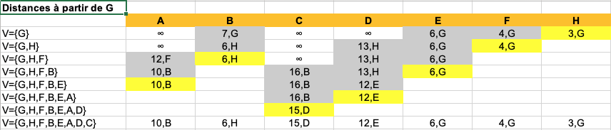
Exercice 1, question 1Exercice 1

# graph.py
#
# A graph is represented as a dictionnary
#  - the keys are the nodes of the graph
#  - the values are the list of nodes adjacent to the key

def nodes(g):
	return list(g.keys())

def neighbors(g, n):
	return g[n]
# bfs.py
#
from graph import *

def breadth_first_search(graph, root):
    visited = []
    tovisit = [root]
    while len(tovisit) != 0 :
        n = tovisit.pop(0)
        if not n in visited:
            for m in neighbors(graph, n):
                if m in visited :
                    continue
                tovisit.append(m)
            visited.append(n)
    return visited
# bfs_depth.py
#
from graph import *

def bfs_depth(graph, root):
    visited = []
    tovisit = [root]
    depth = {root: 0}
    while len(tovisit) != 0 :
        n = tovisit.pop(0)
        if not n in visited:
            for m in neighbors(graph, n):
                if m in visited :
                    continue
                tovisit.append(m)
                if not m in depth :
                    depth[m] = depth[n] + 1
            visited.append(n)
    return depth

#
#     b ---- c
#   /         \
#  a           f
#   \         /
#     d ---- e
#
my_graph = {
  'a': ['b', 'd'],
  'b': ['a', 'c'],
  'c': ['b', 'f'],
  'd': ['a', 'e'],
  'e': ['d', 'f'],
  'f': ['c', 'e']
}

if __name__ == "__main__":
	depth=bfs_depth(my_graph,'a')
	print(depth)

Exercice 1, question 2

Un graphe contient un cycle ayant un nombre impair d'arêtes ssi il existe une arête dont les deux extrémités ont la même profondeur.

On remarque tout d'abord que les profondeurs de deux sommets adjacents d'un graphe diffèrent au maximum de 1. En effet, elles peuvent être égales si les deux sommets sont atteints par des chemins de longueurs égales, mais elles ne peuvent différer de plus de 1 puisque si c'était le cas, en prenant P la profondeur la plus petite, on atteindrait l'autre sommet en P+1 arêtes en suivant l'arête qui relie les deux sommets.

Preuve :
=> on fait la preuve en prenant la contraposée : si toutes les arêtes relient des sommets de profondeurs différentes, le graphe ne contient pas de cycle de longueur impaires. En effet, si toutes les arêtes relient des sommets de profondeurs différentes, ces profondeurs diffèrent toutes de 1. En parcourant le cycle, on alterne donc entre des sommets de profondeur paire et des sommets de profondeur impaire. Pour revenir au sommet de départ (et donc à la même parité pour sa profondeur) dans le parcours du cycle, il faut donc suivre un nombre pair d'arêtes. il ne peut donc pas y avoir de cycle de longueur impaire.

<= s'il existe une arête reliant deux sommets x et y de même profondeur, on recherche l'ancêtre commun r à ces deux sommets (au pire, c'est la racine). Les chemins de r à x et de r à y ont la même longueur L, donc la somme de leurs longueurs, 2L est paire. En ajoutant l'arête qui relie x à y, on obtient un cycle de longueur 2L+1, qui est bien impaire.

Exercice 1, question 3

# has_odd_cycle.py
#
from bfs_depth import *

def has_odd_cycle(g):
	depth = bfs_depth(g, nodes(g)[0])
	for n1 in nodes(g):
		for n2 in neighbors(g, n1):
		  if depth[n1] == depth[n2]:
		  	return True
	return False

#
#     b ---- c
#   /         \
#  a           f
#   \         /
#     d ---- e
#
even_cycles = {
  'a': ['b', 'd'],
  'b': ['a', 'c'],
  'c': ['b', 'f'],
  'd': ['a', 'e'],
  'e': ['d', 'f'],
  'f': ['c', 'e']
}

#
#     b ---- c ---- d
#   /         
#  a                |
#   \               |
#     e ---- f ---- g
#
odd_cycle = {
  'a': ['b', 'e'],
  'b': ['a', 'c'],
  'c': ['b', 'd'],
  'd': ['c', 'g'],
  'e': ['a', 'f'],
  'f': ['e', 'g'],
  'g': ['f', 'd']
}

if __name__ == "__main__":
	print("even", has_odd_cycle(even_cycles))
	print("odd", has_odd_cycle(odd_cycle))

Exercice 1, question 4

Dans un graphe biparti, il ne peut pas exister de cycle ayant un nombre impair d'arêtes.

En effet, toutes les arêtes d'un graphe biparti relient un sommet de V1 à un sommet de V2. Pour fermer un cycle, il faut donc que ce cycle fasse un nombre entier d'aller-retours entre V1 et V2, sa longueur est donc nécessairement paire.

Réciproquement, si un graphe ne contient pas de cycle ayant un nombre impair d'arêtes, il est biparti. En effet, toute arête relie alors des sommets de profondeurs qui diffèrent exactement de 1. Toute arête relie donc un sommet de profondeur paire à un sommet de profondeur impaire. En choisissant pour V1 le sous-ensemble des sommets de profondeur paire, et pour V2 le sous-ensemble des sommets de profondeur impaire, on obtient une partition des sommets en deux sous-ensembles, telle que toute arête relie des sommets appartenant à des sous-ensembles différents.

Exercice 1, question 5

# bipartite.py
#
from bfs_depth import *

def is_bipartite(graph):
    depth = bfs_depth(graph, nodes(graph)[0])
    for v in nodes(graph) :
        for n in neighbors(graph, v) :
            if depth[v] == depth[n] :
                return False
    return True

#
# a --- b --- c --- d
# |  \  |  X  |     |
# e     f --- g --- h
my_graph1 = {
  'a': ['b', 'e', 'f'],
  'b': ['a', 'c', 'f', 'g'],
  'c': ['b', 'd', 'f', 'g'],
  'd': ['c', 'h'],
  'e': ['a'],
  'f': ['a', 'b', 'c', 'g'],
  'g': ['b', 'c', 'f', 'h'],
  'h': ['d', 'g']
}
if __name__ == "__main__":
	print("graph01 is bipartite?", is_bipartite(my_graph1))

Exercice 2, question 1Exercice 1

Un graphe est 2-coloriable ssi il est biparti

En effet, si le graphe est 2-coloriable, on prend pour V1 les sommets de la première couleur, et pour V2 ceux de la deuxième couleur. On a alors une partition des sommets du graphe, et toutes les arêtes relient un sommet de V1 à un sommet de V2 puisque deux sommets adjacents n'ont pas la même couleur.

Réciproquement, si un graphe est biparti, on colore d'une couleur les sommets de V1 et de l'autre couleur les sommets de V2 et on obtient un 2-coloriage du graphe.

Exercice 2, question 2

# dfs.py
#
from graph import *

def depth_first_search_iter(graph, root):
    visited = []
    tovisit = [root]
    while len(tovisit) != 0 :
        n = tovisit.pop(0)
        if not n in visited:
            for m in neighbors(graph, n):
                if m in visited :
                    continue
                tovisit.insert(0,m)
            visited.append(n)
    return visited

#
#     b ---- c
#   /         \
#  a           f
#   \         /
#     d ---- e
#
my_graph = {
  'a': ['b', 'd'],
  'b': ['a', 'c'],
  'c': ['b', 'f'],
  'd': ['a', 'e'],
  'e': ['d', 'f'],
  'f': ['c', 'e']
}

if __name__ == '__main__':
	my_dfs=depth_first_search_iter(my_graph,'a')
	print(my_dfs)
# 2-color.py
#
from graph import *

def two_color_iter(graph, root):
	tovisit = [root]
	colors = {root: 0}
	while len(tovisit) > 0 :
		n = tovisit.pop()
		for m in neighbors(graph, n):
			if m in colors and colors[m] == colors[n] :
				return (False, {})
			if not m in colors:
				colors[m] = 1 - colors[n]
				tovisit.append(m)
	return (True, colors)

def two_color_rec(graph, root):
	return two_color_rec_aux(graph, root, {root: 0})

def two_color_rec_aux(graph, root, colors):
	for m in neighbors(graph, root):
		if m in colors and colors[m] == colors[root] :
			return (False, {})
		if not m in colors:
			colors[m] = 1 - colors[root]
			return two_color_rec_aux(graph, m, colors)
	return (True, colors)

#
#     b ---- c
#   /         \
#  a           f
#   \         /
#     d ---- e
#
my_graph = {
  'a': ['b', 'd'],
  'b': ['a', 'c'],
  'c': ['b', 'f'],
  'd': ['a', 'e'],
  'e': ['d', 'f'],
  'f': ['c', 'e']
}

#
#  a --- b --- c --- d
#  |  \  |  X  |     |
#  e     f --- g --- h
#
graph_ex = {
	'a': ['b', 'e', 'f'],
	'b': ['a', 'c', 'f', 'g'],
	'c': ['b', 'd', 'f', 'g'],
	'd': ['c', 'h'],
	'e': ['a'],
	'f': ['a', 'b', 'c', 'g'],
	'g': ['b', 'c', 'f'],
	'h': ['d', 'g']
}

if __name__ == '__main__':
	print(two_color_iter(my_graph,'a'))
	print(two_color_rec(my_graph,'a'))
	print(two_color_iter(graph_ex, 'a'))
	print(two_color_rec(graph_ex, 'a'))

Exercice 2, question 3

L'algorithme est correct car :

  • quand il rend True, il a parcouru tous les sommets du graphe en donnant une couleur différente aux sommets adjacents, ou en vérifiant que les couleurs sont différentes quand un voisin est déjà coloré.
  • quand il rend False, il a trouvé deux sommets adjacents de même couleur, c'est-à-dire dont les profondeurs ont la même parité. La somme de ces parités est donc paire (car impair + impair -> pair, et pair + pair -> pair). En fermant ces deux chemins avec l'arête qui relie ces sommets, ont obtient donc un cycle de longueur impaire, ce qui signifie que le graphe n'est pas biparti et donc pas 2-coloriable.

Exercice 3

Un graphe orienté sans circuit contient au moins un sommet qui n'a pas d'arc entrant.

On démontre la contraposée : si tous les sommets ont au moins un arc entrant, le graphe contient un cycle.

En effet, prenons un sommet au hasard. Il possède un arc entrant que nous suivons pour arriver à un autre sommet. Ce sommet a également un arc entrant que nous suivons etc. On obtient donc une suite infinie de sommets en remontant les arcs entrant. Or le nombre de sommets du graphe est fini, et cette suite infinie doit donc repasser plusieurs fois par le même sommet. Il y a donc un circuit dans le graphe.

TD n°2

Dessin des graphes pour les différentes questions

import math

def nodes(g) :
  return g.keys()

def neighbours(g, s) :
  return g[s].keys()

def distance(g, s, t) :
  return g[s][t]

hameau = {
    'a': {'b': 4, 'f': 8},
    'b': {'a': 4, 'f': 9, 'g': 7, 'h': 3, 'c': 10, 'd': 12},
    'c': {'b': 10, 'd': 3},
    'd': {'c': 3, 'b': 12, 'h': 10, 'e': 6},
    'e': {'f': 7, 'g': 6, 'h': 3, 'd': 6},
    'f': {'a': 8, 'b': 9, 'g': 4, 'e': 7},
    'g': {'f': 4, 'b': 7, 'h': 3, 'e': 6},
    'h': {'b': 3, 'g': 3, 'd': 10, 'e': 3}
}

# Shortest paths with Dijkstra's algorithm
def dijkstra(graph, start) :
  frontier = set(start)
  state = {v:(math.inf, None) for v in nodes(graph)}  # pairs (distance, parent)
  state[start] = (0, None)

  while len(frontier) > 0 :
    min_node = min(frontier, key=lambda n: state[n][0])
    frontier.remove(min_node)

    for n in neighbours(graph, min_node) :
      # Skip start node, we know its distance is 0
      if n == start :
        continue
      # Compute distance to n when coming from min_node
      new_dist = state[min_node][0] + distance(graph, min_node, n)
      # Add newly touched vertices to the frontier
      if state[n][1] == None:
        frontier.add(n)
        state[n] = (new_dist, min_node) # update distance
      elif new_dist < state[n][0] :  # If the new one is smaller
        state[n] = (new_dist, min_node) # update distance

  return state

print(dijkstra(hameau, 'g'))

# Minimum cost spanning tree with Prim's algorithm
def prim(graph, start) :
  # The initial frontier is the neighbors of the start node
  frontier = set(graph[start].keys())
  # The initial spanning tree has just start as root
  state = {start:(0, None)} # pairs (distance, parent)

  while len(frontier) > 0 :
    # Look for a node in the frontier with a minimal distance to a node of the tree
    (min_node, from_node, min_dist) = (None, None, math.inf)
    for n in frontier :
      for m in graph[n] :
        if m in state and graph[n][m] < min_dist :
          (min_node, from_node, min_dist) = (n, m, graph[n][m])
    # We remove the min node from the frontier
    frontier.remove(min_node)
    # And we add it to the spanning tree
    state[min_node] = (min_dist, from_node)
    # We add the neighbors of the min_node to the frontier
    for n in graph[min_node].keys() :
      if not n in state :
        frontier.add(n)

  return state

# print(prim(hameau, 'g'))

# Minimum cost spanning tree with Kruskal's algorithm
def kruskal(graph):
  # Edges sorted by increasing value
  edges = sorted([(graph[i][j], i, j) \
                    for i in nodes(graph) \
                    for j in neighbours(graph, i) if i < j])

  # Connex components for each node. Initially, each node is in its own component
  components = {i:i for i in graph}
  mst = []

  for e in edges :
    c1 = components[e[1]]
    c2 = components[e[2]]
    if c1 != c2 : # if e connects two different components
      mst.append((e[1], e[2]))  # append it to the MST
      for i in components:  # Update the components
        if components[i] == c2 :
          components[i] = c1
      if len(set(components.values())) == 1 : 
        break
  return mst

# print(kruskal(hameau))

##
# DAGs and topological orders
####
example_dag = {
  'a': {'b': 4, 'c': 2, 'd': 1},
  'b': {'c': 3},
  'c': {'f': 2},
  'd': {'e': 6},
  'e': {'f': 4},
  'f': {}
}
example_dag2 = {
  'a': {'b': 4, 'c': 2},
  'b': {'c': 3},
  'c': {'f': 2},
  'd': {'e': 6},
  'e': {'f': 4},
  'f': {}
}
example_notdag = {
  'a': {'b': 4, 'c': 2},
  'b': {'c': 3},
  'c': {'f': 2},
  'd': {'e': 6},
  'e': {'f': 4},
  'f': {'b': 3}
}

# Find a topological order on a DAG
def topological_order(graph) :
  ordered = []      # ordered vertices
  visited = set()   # already visited vertices
  try :
    for v in nodes(graph) :
      if not v in visited :
        # Depth first search to find the bigger vertices first
        depth_topo(graph, visited, ordered, set(), v)
  except ValueError as err :  # graph is not a DAG
    print(err)
    return None
  # The topological order is the reverse of the order found
  ordered.reverse()
  return ordered

# Depth first search to find vertices ordered from the leaves to the root
def depth_topo(graph, visited, ordered, current_path, v) :
  visited.add(v)        # Remember we went through this vertex
  current_path.add(v)   # Remember this vertex is on the current exploration path
  for u in neighbours(graph, v) :
    if u in current_path :  # If the path crosses itself, we have a cycle!
      raise ValueError("Graph has a cycle")
    if not u in visited :   # Explore only vertices that have not yet been visited
      depth_topo(graph, visited, ordered, current_path, u)
  current_path.remove(v)  # remove vertex from current exploration path
  ordered.append(v)       # append leaf vertex to the end of the order

# Shortest paths relying on topological order
def PCC_topological(graph, start) :
  dist = {v: math.inf for v in nodes(graph)}
  dist[start] = 0

  for v in topological_order(graph) :
    for u in neighbours(graph, v) :
      if dist[u] > dist[v] + distance(graph, v, u) :
        dist[u] = dist[v] +distance(graph, v, u)
  return dist

TD n°3

Dessin des graphes pour les différentes questions

TD n°4

Dessins au tableau pour les différentes questions

# Construit un maillon de la liste chaînée, next est le maillon suivant
# Les maillons sont représentés par des tuples.
def Link(prod, quantity, next) :
	return (prod, quantity, next)

# Construit une liste chaînée vide.
# Une liste chaînée est un tuple à un élément : son premier maillon
# Ceci permet de découpler l'objet liste et son premier maillon (qui peut être amené à 
# changer lors de l'ajout ou de la suppression d'éléments)
# Le premier maillon de la liste vide est None
def LinkedList() :
	return (None,)

# Ajoute un élément à la fin d'une liste.
# Attention, les éléments de la liste sont stockés en ordre inverse
# dans le chaînage afin de faciliter l'ajout d'éléments
def listAppend(list, prod, quantity) :
	return (Link(prod, quantity, list[0]),)

# Affiche un maillon, et récursivement, affiche avant lui 
# tous les maillons qui le suivent. De cette façon, les éléments de la
# liste sont bien affichés dans l'ordre (les derniers maillons en premier.
def printLink(link) :
  if link is None :
    return ""
  linkstr = "(" + link[0] + ", " + str(link[1]) + ")"
  if link[2] is None :
    return linkstr
  else:
    return printLink(link[2]) + ", " + linkstr

# Affiche une liste
def printList(list) :
  return '[' + printLink(list[0]) + ']'

# Programme de test.
def test():
  l = LinkedList()
  print(printList(l))

  l = listAppend(l, 'A', 2)
  print(printList(l))

  l = listAppend(l, 'B', 1)
  print(printList(l))

if __name__ == "__main__":
	test()
stock = [ ('Le Monde', 2),
          ('Le Figaro', 1),
          ('Libération',4),
          ('Les Échos',3),
          ('L\'équipe',5)
]

stock.sort()  # La dichotomie ne fonctionne que si la liste est triée

# Recherche dichotomique dans une liste triée
def dicho_search(stock, prod):
  (begin, end) = (0, len(stock)-1)
  while begin <= end:
    middle = (begin + end) // 2
    if stock[middle][0] == prod:
      return middle
    elif (stock[middle][0] > prod): # lexicographic comparison
      end = middle - 1
    else:
      begin = middle + 1
  return None

# Insertion dichotomique
# Rend None si l'élement est déjà présent
# Rend l'indice où insérer l'élément sinon
def dicho_insert(stock, prod):
  (begin, end) = (0, len(stock)-1)
  while begin <= end:
    middle = (begin + end) //2
    if stock[middle][0] == prod:
      return None
    elif (stock[middle][0] > prod): # comparaison lexicographique
      end = middle - 1
    else:
      begin = middle + 1
  # Si on ajoute à la fin de la liste, il faut placer middle au-delà 
  # de la fin de la liste courante
  if middle == len(stock) - 1 :
    middle += 1
  # On allonge la liste
  stock.append(None)
  # On décale vers la droite les éléments plus grand que celui qu'on va insérer
  for i in range(len(stock)-1, middle, -1):
    stock[i] = stock[i-1]
  return middle

# Accès à la valeur du stock
def get_dicho(stock, prod):
  idx = dicho_search(stock, prod)
  if idx is None :
    return None
  else:
    return stock[idx][1]

# Mise à jour de la valeur du stock
def set_dicho(stock, prod, nb):
  idx = dicho_search(stock, prod)
  if idx is None :
    return None
  else:
    stock[idx] = (prod, nb)
    return nb

# Ajout d'un élément au catalogue
def add_dicho(stock, prod, nb):
  idx = dicho_insert(stock, prod)
  if idx is None :
    return None
  else:
    stock[idx] = (prod, nb)
    return nb

def del_dicho(stock, prod):
  idx = dicho_search(stock, prod)
  if not idx is None :
    del stock[idx]

if __name__ == "__main__":
  print("get_dicho(stock, 'Les Échos')")
  print(get_dicho(stock, 'Les Échos'))

  print("set_dicho(stock, 'Le Monde', 10)")
  set_dicho(stock, 'Le Monde', 10)
  print(stock)

  print("add_dicho(stock, 'Le Z', 42)")
  add_dicho(stock, 'Le Z', 42)
  print(stock)

  print("add_dicho(stock, 'A', 21)")
  add_dicho(stock, 'A', 21)
  print(stock)

  print("add_dicho(stock, 'Z', 84)")
  add_dicho(stock, 'Z', 84)
  print(stock)

  print("del_dicho(stock, 'Le Z')")
  del_dicho(stock, 'Le Z')
  print(stock)

  print("del_dicho(stock, 'A')")
  del_dicho(stock, 'A')
  print(stock)

  print("del_dicho(stock, 'Z')")
  del_dicho(stock, 'Z')
  print(stock)
# Liste chaînée selon une approche objet
# frederic.boulanger@centralesupelec.fr  12/2020

# Classe des listes chaînées
class LinkedList :
  # Classe des maillons, interne à la classe LinkedList
  class __Link :
    # Constructeur de la classe Link
    def __init__(self, value, next = None) :
      self.value = value  # initialisation de la valeur
      self.next = next    # initialisation du maillon suivant

  # Classe des itérateurs sur nos listes
  # Un itérateur permet de parcourir efficacement une liste
  class __Iterator:
    # Constructeur : initialise l'itérateur avec link comme point de départ
    def __init__(self, link):
      self.current = link

    # Cette méthode rend l'élément courant et déplace l'itérateur sur le suivant
    def __next__(self):
      if self.current is None :
        raise StopIteration()
      res = self.current.value
      self.current = self.current.next
      return res

  # Constructeur de liste. Crée une liste vide
  def __init__(self):
    self.first = None

  # Rend un itérateur sur la liste à partir de son 1er élément
  # Permet notamment d'utiliser "for e in list" avec nos listes
  def __iter__(self):
    return self.__Iterator(self.first)

  # Rend la longueur de la liste
  def length(self):
    l = 0
    cur = self.first
    while cur is not None :
      l += 1
      cur = cur.next
    return l

  # Permet d'utiliser la fonction "len" sur nos listes
  def __len__(self) :
    return self.length()

  # Ajoute un élément en tête de liste
  def prepend(self, value):
    self.first = self.__Link(value, self.first)

  # Ajoute un élément à la fin de la liste
  def append(self, value):
    if self.first is None :
      self.first = self.__Link(value)
      return
    cur = self.first
    while cur.next != None :
      cur = cur.next
    cur.next = self.__Link(value)

  # Concatène une liste à celle-ci
  def concat(self, list):
    for item in list :
      self.append(item)

  # Permet d'utiliser "+" pour la concaténation
  def __add__(self, list) :
    self.concat(list)

  # Rend l'élément à l'indice "index"
  def get(self, index) :
    idx = 0
    cur = self.first
    while cur != None :
      if idx == index :
        return cur.value
      cur = cur.next
      idx += 1
    return None

  # Permet d'utiliser la notation list[i] pour accéder à l'élément d'incice i
  def __getitem__(self, index) :
    return self.get(index)

  # Change la valeur de l'élément d'indice "index"
  def set(self, index, value) :
    idx = 0
    cur = self.first
    while cur != None :
      if idx == index :
        cur.value = value
        return
      cur = cur.next
      idx += 1

  # Permet d'utiliser la notation "list[i] = (p, n)" à la place de "set"
  def __setitem__(self, index, value) :
    self.set(index, value)

  # Supprime l'élement d'indice "index"
  def remove(self, index) :
    idx = 0
    prev = None
    cur = self.first
    while cur != None :
      if idx == index :
        if prev == None :
          self.first = cur.next
        else :
          prev.next = cur.next
        return
      prev = cur
      cur = cur.next
      idx += 1

  # Permet d'utiliser la notation "del list[i]" à la place de "remove"
  def __delitem__(self, index) :
    return self.remove(index)

  # Supprime tous les éléments dont la valeur est "value" de la liste
  def removeValue(self, value) :
    prev = None
    cur = self.first
    while cur != None :
      if cur.value == value :
        if prev == None :
          self.first = cur.next
        else :
          prev.next = cur.next
      else:
        prev = cur
      cur = cur.next

  # Construit une représentation de la liste sous forme d'une chaîne de caractères
  # Permet d'utiliser la fonction "str", ou de passer une liste à la fonction "print"
  def __str__(self) :
    res = '['
    cur = self.first
    while cur != None :
      if cur != self.first :
        res += ', '
      res += str(cur.value)
      cur = cur.next
    res += ']'
    return res

# Une classe pour représenter les stocks de journaux
class Journal:
  def __init__(self, nom, nb) :
    self.nom = nom
    self.nb = nb

  # Deux stocks de journaux sont égaux s'ils ont le même nom de journal 
  # et le même nombre d'exemplaires
  def __eq__(self, j) :
    return self.nom == j.nom and self.nb == j.nb

  def __str__(self) :
    return '(' + self.nom + ': ' + str(self.nb) +')'

# Programme de test
def test():
  l = LinkedList()

  l.append(Journal("Le Monde", 2))
  print(l)

  l.append(Journal("Le Figaro", 1))
  print(l)

  l.prepend(Journal("Libération", 3))
  print(l)

  l.prepend(Journal("Les Échos", 4))
  print(l)

  # Test de l'accès avec __getitem__
  l[1].nb = 5
  print(l)

  # Test de la modification avec __setitem__
  l[3] = Journal("L'Équipe", 6)
  print(l)

  # Test de la suppression avec del
  del l[0]
  print(l)

  # Test de removeValue
  l.removeValue(Journal("Le Monde", 2))
  print(l)

  # Création d'un doublon et test de removeValue dans ce cas
  l.prepend(Journal("L'Équipe", 6))
  print(l)
  l.removeValue(Journal("L'Équipe", 6))
  print(l)

if __name__ == "__main__":
  test()

TD n°6

Dessins au tableau pour les différentes questions

# Example
U = {'A', 'B', 'C', 'D', 'E'}
S = [{'A', 'B'}, {'C', 'D'}, {'D', 'E'}, {'A', 'B', 'C'}]

Sol1 = {0, 1, 2}
Sol2 = {0, 2}
Sol3 = {2, 3}
Sol4 = {1, 42}

def check_setcover(U, S, k, Sol):
	if len(Sol) > k :
		print(f"# Solution {Sol} is too large")
		return False
	for s in Sol :
		if s >= len(S) :
			print(f"# Element {s} of {Sol} is out of range")
			return False
	u = set()
	for idx in Sol :
		u.update(S[idx])
	if u != U :
		print(f"# Solution {Sol} covers only {u}")
		return False
	return True

print("Sol1", check_setcover(U, S, 2, Sol1))
print("Sol2", check_setcover(U, S, 2, Sol2))
print("Sol3", check_setcover(U, S, 2, Sol3))
print("Sol4", check_setcover(U, S, 2, Sol4))

TD n°7

Dessins au tableau pour les différentes questions

weights = [4, 4, 5, 5, 5, 4, 4, 6, 6, 2, 2, 3, 3, 7, 7, 2, 2, 5, 5, 8, 8, 4, 4, 5]
capacity = 10

def check_packing(items, bags, capacity, max_bags) :
  if len(bags) > max_bags :
    return False
  packed_items = [item for bag in bags for item in bag]
  if sorted(items) != sorted(packed_items) :
    return False
  for bag in bags :
    if sum(bag) > capacity :
      return False
  return True

# O(n)
def NextFit(items, capacity) :
  bags = [[]]
  for item in items :
    if sum(bags[-1]) + item > capacity :
      bags.append([item])
    else :
      bags[-1].append(item)
  return bags

# O(n^2)
def FirstFit(items, capacity) :
  bags = []
  for item in items :
    placed = False
    for bag in bags :
      if sum(bag) + item <= capacity :
        placed = True
        bag.append(item)
        break
    if not placed :
      bags.append([item])
  return bags

# O(n^2)
def FirstFitDecreasing(items, capacity) :
  return FirstFit(sorted(items, reverse=True), capacity)

# O(n^2)
def BestFit(items, capacity):
  bags = []
  for item in items :
    best_bag = None
    min_space = None
    for idx in range(len(bags)):
      space = capacity - sum(bags[idx])
      if item <= space and (min_space is None or space < min_space) :
        best_bag = idx
        min_space = space
    if best_bag is None:
      bags.append([item])
    else:
      bags[best_bag].append(item)
  return bags

# O(n^2)
def BestFitDecreasing(items, capacity) :
  return BestFit(sorted(items, reverse=True), capacity)

for algo in [NextFit, FirstFit, BestFit, FirstFitDecreasing, BestFitDecreasing] :
  bags = algo(weights, capacity)
  print(algo.__name__)
  print(bags)
  print("# bags = ", len(bags),
        ", check packing: ", check_packing(weights, bags, capacity, len(bags)))
  print()

TD pratique n°8

Explications au tableau

# Small instance for debugging
W4 = 5                                                    # weight limit of the knapsack
O4 = { 'o1': {'w': 1, 'v': 10}, 'o2': {'w': 2, 'v': 20},  # 'w' for weight and 'v' for value
       'o3': {'w': 3, 'v': 15}, 'o4': {'w': 4, 'v': 20} }


# a bigger instance of  Knapsack with 15 objects
W15 = 750                             
O15 = { 'o1':  {'w': 70,  'v': 135}, 'o2':  {'w': 73,  'v': 139}, 'o3':  {'w': 77,  'v': 149}, 
        'o4':  {'w': 80,  'v': 150}, 'o5':  {'w': 82,  'v': 156}, 'o6':  {'w': 87,  'v': 163}, 
        'o7':  {'w': 90,  'v': 173}, 'o8':  {'w': 94,  'v': 184}, 'o9':  {'w': 98,  'v': 192}, 
        'o10': {'w': 106, 'v': 201}, 'o11': {'w': 110, 'v': 210}, 'o12': {'w': 113, 'v': 214}, 
        'o13': {'w': 115, 'v': 221}, 'o14': {'w': 118, 'v': 229}, 'o15': {'w': 120, 'v': 240} }

"""
Data structure for an instance of the knapsack problem
"""
def knapsack(obj_dict, obj_list, max_weight):
  return {
    'dict': obj_dict,  # dictionary of objects weight and value
    'list': obj_list,  # list of objects in traversal order
    'maxW': max_weight # maximum allowed weight in the knapsack
  }

"""
Data structure for a solution to the knapsack problem
"""
def solution(selected, next, weight, value):
  return {
    'selected': selected,  # objects selected to be in the knapsack
    'next':     next,      # index of the next object to consider
    'weight':   weight,    # total weight of the objects in the knapsack
    'score':    value      # total value of the objects in the knapsack
  }

###
# Utility functions
###
"""Get object at a given index"""
def object(knapsack, index):
  return knapsack['list'][index]

"""Get the weight of an object"""
def weight(knapsack, object):
  return knapsack['dict'][object]['w']

"""Get the value of an object"""
def value(knapsack, object):
  return knapsack['dict'][object]['v']

"""
Check if the next object fits into the knapsack
"""
def next_does_fit(knapsack, sol):
  return sol['weight'] + weight(knapsack, object(knapsack, sol['next'])) <= knapsack['maxW']

"""
Build the next solution without taking the next object
"""
def sol_without_next(knapsack, sol):
  # To be completed

"""
Build the next solution when taking the next object
"""
def sol_with_next(knapsack, sol):
  # To be completed

###
# Backtracking algorithm
###
"""
Find the optimal solution to the knapsack problem by exploring all possible solutions
"""
def backtracking(obj_dict, max_weight) :
  """
  Compute the children of the current partial solution
  """
  def children(knapsack, cursol):
    children = []
    # To be completed
    return children

  """
  Tell if a solution is terminal, i.e. there are no more objects to consider
  """
  def terminal(knapsack, cursol):
    return cursol['next'] == len(knapsack['list'])

  """
  Explore solutions starting from cursol, and return the best one, knowing
  that the current best solution is "best".
  """
  def backtracking_rec(knapsack, cursol, best) :
    if terminal(knapsack, cursol) :
      # If the current solution is terminal, check if it is better that the current best one
      if best is None or cursol['score'] > best['score']  :
        return cursol
    else :
      # If the solution is not terminal, recursively explore its children
      for sol in children(knapsack, cursol):
        best = backtracking_rec(knapsack, sol, best)
    # Return the best solution so far
    return best

  # Build the instance of the problem
  instance = knapsack(obj_dict, sorted(obj_dict.keys()), max_weight)
  # And start exploring from the empty partial solution
  rootsol = solution(set(), 0, 0, 0)
  return backtracking_rec(instance, rootsol, None)


def test_backtracking():
  print()
  print('-- BACKTRACKING --') 
  bestSol4 = backtracking(O4, W4)
  selected = bestSol4['selected']
  score = bestSol4['score']
  print(f'--- simple case : 4 objects --- best found solution {selected} of value {score}')
  assert score == 35
  assert selected == {'o2', 'o3'}

  bestSol15 = backtracking(O15, W15)
  selected = bestSol15['selected']
  score = bestSol15['score']
  print(f'--- bigger case : 15 objects --- best found solution {selected} of value {score}')
  assert score == 1458
  assert selected == {'o1', 'o3', 'o5', 'o7', 'o8', 'o9', 'o14', 'o15'}

test_backtracking()

###
# Branch & Bound
###
"""
Find the optimal solution to the knapsack problem by branching and bounding the solution tree
"""
def branchbound(obj_dict, max_weight) :
  """
  Tell if we should cut the branch because it cannot lead to a better solution
  """
  def bound(knapsack, sol, best) :
    if best is None :
      return False  # Don't cut the branch when there is no best solution
    # To be completed

  """
  Compute the children of the current partial solution
  """
  def children(knapsack, cursol, best):
    children = []
    # To be completed

  """
  Tell if a partial solution is terminal, i.e. there is no more objects to consider
  """
  def terminal(knapsack, cursol):
    return cursol['next'] == len(knapsack['list'])

  """
  Explore solutions starting from cursol, and return the best one, knowing
  that the current best solution is "best".
  """
  def branchbound_rec(knapsack, cursol, best) :
    if terminal(knapsack, cursol) :
      if best is None or cursol['score'] > best['score']  :
        return cursol
    else :
      for sol in children(knapsack, cursol, best):
        best = branchbound_rec(knapsack, sol, best)
    return best

  # Prepare the instance with the objects sorted in descending order of value density
  instance = knapsack(obj_dict,
                      # To be completed
                      max_weight)
  # And start exploring from the empty partial solution
  rootsol = solution(set(), 0, 0, 0)
  return branchbound_rec(instance, rootsol, None)

def test_branch_bound():
  print()
  print('-- Branch & bound --')
  bestSol4 = branchbound(O4, W4)
  selected = bestSol4['selected']
  score = bestSol4['score']
  print(f'--- simple case : 4 objects --- best found solution {selected} of value {score}')
  assert score == 35
  assert selected == {'o2', 'o3'}

  bestSol15 = branchbound(O15, W15)
  selected = bestSol15['selected']
  score = bestSol15['score']
  print(f'--- bigger case : 15 objects --- best found solution {selected} of value {score}')
  assert score == 1458
  assert selected == {'o1', 'o3', 'o5', 'o7', 'o8', 'o9', 'o14', 'o15'}

test_branch_bound()

### Dynamic programming
def knapsack_dyn(obj_dict, max_weight):
  obj_list = sorted(obj_dict.keys())
  n = len(obj_list)
  # Initialize the matrix of optimal values
  v = [ [0 for j in range(max_weight + 1)] for i in range(n + 1)]
  # Fill the matrix using the recurrence relations

  # To be completed

  # Now, rebuild the solution
  selected = set()
  # Start from the last object and maximum weight
  i = n-1
  w = max_weight
  while i >= 0 :
    # To be completed

  # Compute the weight of the solution
  weight = 0
  for o in selected :
    weight += obj_dict[o]['w']
  # Return the solution in the same form as the other algorithms
  return solution(selected, n, weight, v[n][max_weight])

def test_prog_dyn():
  print()
  print('-- Programmation dynamique --')
  bestSol4 = knapsack_dyn(O4, W4)
  selected = bestSol4['selected']
  score = bestSol4['score']
  print(f'--- simple case : 4 objects --- best found solution {selected} of value {score}')
  assert score == 35
  assert selected == {'o2', 'o3'}

  bestSol15 = knapsack_dyn(O15, W15)
  selected = bestSol15['selected']
  score = bestSol15['score']
  print(f'--- bigger case : 15 objects --- best found solution {selected} of value {score}')
  assert score == 1458
  assert selected == {'o1', 'o3', 'o5', 'o7', 'o8', 'o9', 'o14', 'o15'}

test_prog_dyn()

############## Comparing the different algorithms ##################
import matplotlib.pyplot as plt
from timeit import timeit
from random import randint

"""
Build some random instance of size n
"""
def random_instance(n):
  max_vw = n**2  # Arbitrary max value for weight and value
  objects = {f'o{i}': {'w': randint(1, max_vw), 'v': randint(1, max_vw)} for i in range(1, n+1)}
  return (max_vw, objects)

"""
Compare the execution time of the three algorithms
"""
def benchmark():
  time_basic = []
  time_branching = []
  time_dyn = []

  n_list = []

  print()
  print("-- Benchmark --")

  for n in range(30, 50):
    n_list.append(n)
    print("# Random instances of size ", n)

    t_back = 0
    t_branch = 0
    t_dyn = 0
    # Average execution time over some number of random instances of the same size
    nb_inst = 4
    for i in range(nb_inst):
      # generate a random instance of size n
      (max_weight, obj_dict) = random_instance(n)
      t_back += timeit(lambda: backtracking(obj_dict, max_weight), number=1) / nb_inst
      t_branch += timeit(lambda: branchbound(obj_dict, max_weight), number=1) / nb_inst
      t_dyn += timeit(lambda: knapsack_dyn(obj_dict, max_weight), number=1) / nb_inst
    time_basic.append(t_back)
    time_branching.append(t_branch)
    time_dyn.append(t_dyn)

  plt.xlabel('N')
  plt.ylabel('T')
  plt.plot(n_list, time_basic, 'r^', label='backtracking')
  plt.plot(n_list, time_branching, 'b^', label='branch & bound')
  plt.plot(n_list, time_dyn, 'g^', label='dynamic prog.')

  plt.legend()
  plt.show()

benchmark()
# Small instance for debugging
W4 = 5                                                    # weight limit of the knapsack
O4 = { 'o1': {'w': 1, 'v': 10}, 'o2': {'w': 2, 'v': 20},  # 'w' for weight and 'v' for value
       'o3': {'w': 3, 'v': 15}, 'o4': {'w': 4, 'v': 20} }


# a bigger instance of  Knapsack with 15 objects
W15 = 750                             
O15 = { 'o1':  {'w': 70,  'v': 135}, 'o2':  {'w': 73,  'v': 139}, 'o3':  {'w': 77,  'v': 149}, 
        'o4':  {'w': 80,  'v': 150}, 'o5':  {'w': 82,  'v': 156}, 'o6':  {'w': 87,  'v': 163}, 
        'o7':  {'w': 90,  'v': 173}, 'o8':  {'w': 94,  'v': 184}, 'o9':  {'w': 98,  'v': 192}, 
        'o10': {'w': 106, 'v': 201}, 'o11': {'w': 110, 'v': 210}, 'o12': {'w': 113, 'v': 214}, 
        'o13': {'w': 115, 'v': 221}, 'o14': {'w': 118, 'v': 229}, 'o15': {'w': 120, 'v': 240} }

"""
Data structure for an instance of the knapsack problem
"""
def knapsack(obj_dict, obj_list, max_weight):
  return {
    'dict': obj_dict,  # dictionary of objects weight and value
    'list': obj_list,  # list of objects in traversal order
    'maxW': max_weight # maximum allowed weight in the knapsack
  }

"""
Data structure for a solution to the knapsack problem
"""
def solution(selected, next, weight, value):
  return {
    'selected': selected,  # objects selected to be in the knapsack
    'next':     next,      # index of the next object to consider
    'weight':   weight,    # total weight of the objects in the knapsack
    'score':    value      # total value of the objects in the knapsack
  }

###
# Utility functions
###
"""Get object at a given index"""
def object(knapsack, index):
  return knapsack['list'][index]

"""Get the weight of an object"""
def weight(knapsack, object):
  return knapsack['dict'][object]['w']

"""Get the value of an object"""
def value(knapsack, object):
  return knapsack['dict'][object]['v']

"""
Check if the next object fits into the knapsack
"""
def next_does_fit(knapsack, sol):
  return sol['weight'] + weight(knapsack, object(knapsack, sol['next'])) <= knapsack['maxW']

"""
Build the next solution without taking the next object
"""
def sol_without_next(knapsack, sol):
  return solution(
          sol['selected'],
          sol['next'] + 1,
          sol['weight'],
          sol['score']
         )

"""
Build the next solution when taking the next object
"""
def sol_with_next(knapsack, sol):
  next_obj = object(knapsack, sol['next'])
  return solution(
          sol['selected'] | {next_obj},
          sol['next'] + 1,
          sol['weight'] + weight(knapsack, next_obj),
          sol['score'] + value(knapsack, next_obj)
         )

###
# Backtracking algorithm
###
"""
Find the optimal solution to the knapsack problem by exploring all possible solutions
"""
nb_calls = 0

def backtracking(obj_dict, max_weight) :
  """
  Compute the children of the current partial solution
  """
  def children(knapsack, cursol):
    children = []
    if terminal(knapsack, cursol):
      # If there are no more objects to consider
      return children
    if next_does_fit(knapsack, cursol):
      # If the next object fits into the knapsack, add the solution with that object
      children.append(sol_with_next(knapsack, cursol))
    # Finally, add the solution without that object
    children.append(sol_without_next(knapsack, cursol))
    return children

  """
  Tell if a solution is terminal, i.e. there are no more objects to consider
  """
  def terminal(knapsack, cursol):
    return cursol['next'] == len(knapsack['list'])

  """
  Explore solutions starting from cursol, and return the best one, knowing
  that the current best solution is "best".
  """
  def backtracking_rec(knapsack, cursol, best) :
    global nb_calls
    nb_calls += 1
    if terminal(knapsack, cursol) :
      # If the current solution is terminal, check if it is better that the current best one
      if best is None or cursol['score'] > best['score']  :
        return cursol
    else :
      # If the solution is not terminal, recursively explore its children
      for sol in children(knapsack, cursol):
        best = backtracking_rec(knapsack, sol, best)
    # Return the best solution so far
    return best

  global nb_calls
  nb_calls = 0
  # Build the instance of the problem
  instance = knapsack(obj_dict, sorted(obj_dict.keys()), max_weight)
  # And start exploring from the empty partial solution
  rootsol = solution(set(), 0, 0, 0)
  return backtracking_rec(instance, rootsol, None)

def test_backtracking():
  print()
  print('-- BACKTRACKING --') 
  bestSol4 = backtracking(O4, W4)
  selected = bestSol4['selected']
  score = bestSol4['score']
  print(f'--- simple case : 4 objects --- best found solution {selected} of value {score}')
  print(f'--  nb calls = {nb_calls}')
  assert score == 35
  assert selected == {'o2', 'o3'}

  bestSol15 = backtracking(O15, W15)
  selected = bestSol15['selected']
  score = bestSol15['score']
  print(f'--- bigger case : 15 objects --- best found solution {selected} of value {score}')
  print(f'--  nb calls = {nb_calls}')
  assert score == 1458
  assert selected == {'o1', 'o3', 'o5', 'o7', 'o8', 'o9', 'o14', 'o15'}

test_backtracking()

###
# Branch & Bound
###
"""
Find the optimal solution to the knapsack problem by branching and bounding the solution tree
"""
def branchbound(obj_dict, max_weight) :
  """
  Tell if we should cut the branch because it cannot lead to a better solution
  """
  def bound(knapsack, sol, best) :
    if best is None :
      return False  # Don't cut the branch when there is no best solution
    # Remaining objects to consider
    remaining = range(sol['next'], len(knapsack['list']))
    w = sol['weight']
    v = sol['score']
    for i in remaining :
    	o = object(knapsack, i)
    	w += weight(knapsack, o)
    	v += value(knapsack, o)
    	if w > knapsack['maxW'] :
    		break
    return v < best['score']

  """
  Compute the children of the current partial solution
  """
  def children(knapsack, cursol, best):
    children = []
    if terminal(knapsack, cursol):
      # If there are no more objects to consider
      return children
    if next_does_fit(knapsack, cursol) \
       and not bound(knapsack, cursol, best):
      # If the next object fits into the knapsack, 
      # and if it not impossible to reach a better solution than best,
      # add the solution with that object
      children.append(sol_with_next(knapsack, cursol))
    # Finally, add the solution without that object
    children.append(sol_without_next(knapsack, cursol))
    return children

  """
  Tell if a partial solution is terminal, i.e. there is no more objects to consider
  """
  def terminal(knapsack, cursol):
    return cursol['next'] == len(knapsack['list'])

  """
  Explore solutions starting from cursol, and return the best one, knowing
  that the current best solution is "best".
  """
  def branchbound_rec(knapsack, cursol, best) :
    global nb_calls
    nb_calls += 1
    if terminal(knapsack, cursol) :
      if best is None or cursol['score'] > best['score']  :
        return cursol
    else :
      for sol in children(knapsack, cursol, best):
        best = branchbound_rec(knapsack, sol, best)
    return best

  global nb_calls
  nb_calls = 0
  # Prepare the instance with the objects sorted in descending order of value density
  instance = knapsack(obj_dict,
                      sorted(obj_dict.keys(),
                      			 key = lambda o : obj_dict[o]['v'] / obj_dict[o]['w'],
                      			 reverse = True),
                      max_weight)
  # And start exploring from the empty partial solution
  rootsol = solution(set(), 0, 0, 0)
  return branchbound_rec(instance, rootsol, None)

def test_branch_bound():
  print()
  print('-- Branch & bound --')
  bestSol4 = branchbound(O4, W4)
  selected = bestSol4['selected']
  score = bestSol4['score']
  print(f'--- simple case : 4 objects --- best found solution {selected} of value {score}')
  print(f'--  nb calls = {nb_calls}')
  assert score == 35
  assert selected == {'o2', 'o3'}

  bestSol15 = branchbound(O15, W15)
  selected = bestSol15['selected']
  score = bestSol15['score']
  print(f'--- bigger case : 15 objects --- best found solution {selected} of value {score}')
  print(f'--  nb calls = {nb_calls}')
  assert score == 1458
  assert selected == {'o1', 'o3', 'o5', 'o7', 'o8', 'o9', 'o14', 'o15'}

test_branch_bound()

### Dynamic programming
def knapsack_dyn(obj_dict, max_weight):
  obj_list = sorted(obj_dict.keys())
  n = len(obj_list)
  # Initialize the matrix of optimal values
  v = [ [0 for j in range(max_weight + 1)] for i in range(n + 1)]
  # Fill the matrix using the recurrence relations
  for i in range(1, n+1):
    obj = obj_list[i - 1]
    weight = obj_dict[obj]['w']
    value = obj_dict[obj]['v']
    for j in range(1, max_weight+1):
      if j < weight :
        v[i][j] = v[i-1][j]
      else:
        v[i][j] = max(v[i-1][j], v[i-1][j-weight] + value)

  # Now, rebuild the solution
  selected = set()
  # Start from the last object and maximum weight
  i = n-1
  w = max_weight
  while i >= 0 :
    if v[i+1][w] != v[i][w] :
      # If the value changed between i and i+1, object i has been selected
      selected.add(obj_list[i])
      w -= obj_dict[obj_list[i]]['w']
    i -= 1

  # Compute the weight of the solution
  weight = 0
  for o in selected :
    weight += obj_dict[o]['w']
  # Return the solution in the same form as the other algorithms
  return solution(selected, n, weight, v[n][max_weight])

def test_prog_dyn():
  print()
  print('-- Programmation dynamique --')
  bestSol4 = knapsack_dyn(O4, W4)
  selected = bestSol4['selected']
  score = bestSol4['score']
  print(f'--- simple case : 4 objects --- best found solution {selected} of value {score}')
  assert score == 35
  assert selected == {'o2', 'o3'}

  bestSol15 = knapsack_dyn(O15, W15)
  selected = bestSol15['selected']
  score = bestSol15['score']
  print(f'--- bigger case : 15 objects --- best found solution {selected} of value {score}')
  assert score == 1458
  assert selected == {'o1', 'o3', 'o5', 'o7', 'o8', 'o9', 'o14', 'o15'}

test_prog_dyn()


############## Comparing the different algorithms ##################
import matplotlib.pyplot as plt
from timeit import timeit
from random import randint

"""
Build some random instance of size n
"""
def random_instance(n):
  max_vw = n**2  # Arbitrary max value for weight and value
  objects = {f'o{i}': {'w': randint(1, max_vw), 'v': randint(1, max_vw)} for i in range(1, n+1)}
  return (max_vw, objects)

"""
Compare the execution time of the three algorithms
"""
def benchmark():
  time_basic = []
  time_branching = []
  time_dyn = []

  n_list = []

  print()
  print("-- Benchmark --")

  for n in range(30, 50):
    n_list.append(n)
    print("# Random instances of size ", n)

    t_back = 0
    t_branch = 0
    t_dyn = 0
    # Average execution time over some number of random instances of the same size
    nb_inst = 4
    for i in range(nb_inst):
      # generate a random instance of size n
      (max_weight, obj_dict) = random_instance(n)
      t_back += timeit(lambda: backtracking(obj_dict, max_weight), number=1) / nb_inst
      t_branch += timeit(lambda: branchbound(obj_dict, max_weight), number=1) / nb_inst
      t_dyn += timeit(lambda: knapsack_dyn(obj_dict, max_weight), number=1) / nb_inst
    time_basic.append(t_back)
    time_branching.append(t_branch)
    time_dyn.append(t_dyn)

  plt.xlabel('N')
  plt.ylabel('T')
  plt.plot(n_list, time_basic, 'r^', label='backtracking')
  plt.plot(n_list, time_branching, 'b^', label='branch & bound')
  plt.plot(n_list, time_dyn, 'g^', label='dynamic prog.')

  plt.legend()
  plt.show()

benchmark()